| | | Acoustics & Vib. Lab. | | | |
|
ME 408 - Modal Analysis : Theory and Experiment
Modal analysis is the process of extracting the dynamics characteristics of a vibrating system from experimental transfer functions. The dynamic characteristics of interest are the mode shapes and the modal parameters. A mode shape is the characteristic deformation shape defined by relative amplitudes of the extreme positions of vibration of a system at a single natural frequency. The modal parameters are the natural frequencies, damping ratios, and modal masses associated with each of the mode shapes. The mode shape is a global property of an elastic system. That is the mode shape is associated with a specific natural frequency and damping ratio which can be extracted from almost any system transfer function. A transfer function is a measure of the response of a system to a given input. In vibration analysis, the input is usually a force and the response measured is usually a motion, either displacement, velocity, or acceleration. In order to obtain a transfer function, a known force is applied at one point and the acceleration, for example, is measured at another point. The transfer function can then be obtained by taking the ratio of the two measurements. Six different transfer functions can be defined depending on the type of response measured. The six types are listed below.
When the input and response are measured at the same point, the transfer function is called a driving point transfer function. When the input and response are measured at different points, a spatial transfer function is obtained. In modal analysis the transfer functions are usually obtained using a digital test system. The input and response measurements are digitized and then processed using fast Fourier transform techniques. The transfer function is calculated and stored as a finite number of data points. If any one of the six transfer functions listed above is obtained in this manner, any of the other transfer functions can be obtained through mathematical manipulation of the existing transfer function. Once the transfer functions are obtained, a modal analysis can be performed. There are basically two levels of sophistication available in modal analysis. In the first level, only the natural frequencies and mode shapes are obtained. From this information, "pictures" of how the system is vibrating at its different natural frequencies can be determined and animated for better visualization. For the second level of sophistication, in addition to the natural frequencies and mode shapes, the modal damping ratios and modal masses are also obtained. When all of these parameters have been obtained, a complete mathematical model of the system can be defined. The mathematical model may then be used in computer simulations to predict the response of the system when it is modified. A designer can now evaluate different design modifications without building prototypes. In order to understand how mode shapes and modal parameters can be obtained from transfer functions, it is necessary to consider a specific transfer function. We'll begin with a single degree of freedom system. The system differential equation is obtained using Newton's law: Sum of the forces acting on the mass is equal to the mass times its acceleration.
Because the transfer function is defined in the frequency domain, a sinusoidal forcing function of the form
f(t) = Fejw
t and a solution of the form x(t) = Xeiw
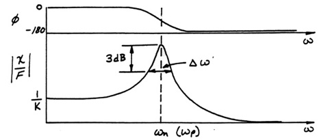
t will be assumed where i = By substituting in the assumed values and dividing out the time varying term (eiw t), the following equation is obtained. The equation can be solved for where: This equation can also be represented as a magnitude and a phase angle. If the magnitude and phase are plotted as a function of frequency, a bode plot is obtained. The bode plot for this system is shown below for a small nonzero damping value.
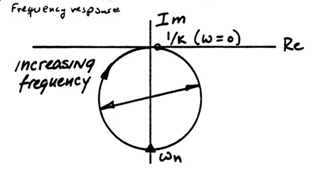
The transfer function can also be separated into real and imaginary parts. If the imaginary part of the transfer function is plotted as a function of the real part, a polar plot (argand plot) is obtained. This plot has the form of a circle.
If the real and imaginary parts are plotted as functions of frequency the coincident and quadrature responses are obtained, respectively.
All of these plots are important in modal analysis and will be used to demonstrate various methods for calculating natural frequencies, damping ratios, masses, and mode shapes. The methods for extracting these parameters will be discussed with reference to the two levels of sophistication mentioned earlier. For the first level of sophistication, the parameters of interest are the natural frequencies and the mode shapes. For a single degree of freedom system there is only one natural frequency and the mode shape for this natural frequency can be viewed as the amplitude of the transfer function at the natural frequency. The natural frequency can be approximated using either the coincident response or the bode plot. For the coincident response, the natural frequency occurs at the frequency where the real part is zero. (See Figure 3). Using the bode plot, the natural frequency can be obtained by determining the peak frequency and recalling that for a compliance transfer function: If the damping ratio is small (
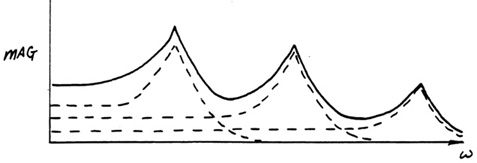
The amplitude at the natural frequency is obtained from the quadrature response by measuring the height of the peak. (See Figure 4) For the second level of sophistication, all of the modal parameters must be obtained. Because these parameters are used in the formulation of a mathematical model of the system, the accuracy of the estimations is very important. For this type of analysis, the designer must use a modal analysis computer program. The modal analysis program uses more sophisticated mathematical techniques for parameter estimation so that, when used properly, more accurate results are obtained. For obtaining natural frequencies and damping ratios, most computer programs use a least squares curve fitting routine to curve fit the transfer function. A solution of the form is assumed and the parameters are varied using an iterative approach until a good fit is obtained. The values of A, w n, and x are then known. For a single degree of freedom system A=1/k. The mass can then be obtained using the definition of the natural frequency. As was mentioned earlier, the amplitude can be obtained from the quadrature response, but it can also be obtained from the polar plot. In the real and imaginary coordinate system, as the frequency increases (from zero to infinity for a single degree of freedom system), the transfer function maps out a circle. The diameter of this circle is the same as the peak amplitude of the quadrature response. With a modal analysis program the amplitude can be determined with greater accuracy by using a circular least squares curve fitting routine to curve fit the circle in the polar plot. A solution of the form (x + a)2 + (y + b)2 = r2 is assumed. The parameters are varied until a good fit is obtained. The diameter can then be calculated. The analysis of a single degree of freedom system can be extended to the analysis of a multi-degree of freedom system. For a linear system, the multi-degree of freedom transfer function can be represented as the sum of single degree of freedom transfer functions. (See Figure 5) The multi-degree of freedom transfer function can be represented in equation form as where:
measured at point K for the rth mode This equation shows that the transfer function can be represented mathematically if the mode shapes, modal masses, natural frequencies, and damping ratios are known. If light damping and widely spaced peaks occur in the transfer function (se Figure 6), the simple parameter estimation techniques can be used for the level one modal analysis. If the peaks are closely spaced or if heavy damping exist (see Figure 7), the more sophisticated techniques for parameter estimation should be used. If a complete mathematical model is desired, the more sophisticated techniques must be used.
To perform a modal analysis of a multi-degree of freedom system, the designer must first obtain a set of system transfer functions. The number and location of the test points depends on the particular system being analyzed. Once the transfer functions have been obtained, the modal parameters can be estimated using the appropriate methods. Because the natural frequencies and damping ratios are global properties, they will be the same for all of the transfer functions. Therefore, these parameters could be estimated from any one of the system transfer functions. Having obtained the parameters of interest, the mode shapes can now be calculated. Figure 8 shows how the mode shapes, of a simple beam, could be obtained using the quadrature response. The mode shapes for the simple beam are shown in Figure 9. The same mode shapes would have been obtained using the circle fitting technique. The points where the mode shapes cross the horizontal axis are called nodes. These are points where there is no motion. If one of the test points is at a node for one of the modes, the peak for that mode will not show up in the transfer function. Therefore, when estimating natural frequencies and damping ratios, a transfer function should be selected in which all the modes are present.
The points where the displacement is the largest are called antinodes. Once the modal parameters and the mode shapes have been determined, the dynamic characteristics of the system can be completely defined. This information could then be used to improve the system or to simply correct an existing problem. Either way, modal analysis provides the designer with a powerful tool for the dynamic analysis and design of mechanical systems.
Euler-Bernoulli Thin Beam Theory A simply supported beam driven by a line force f(t) located at x = xs. System Equation from Newton's Law. To get the transfer function, assume that f(t) is harmonic with frequency w
such that f(t) = Fejw
t where j = If we multiply the equation of motion by
Thus, if the beam transverse displacement is measured at xr, then its response will be: Modal Analysis We define the above ratio as the frequency response function Hrs(w ) = V(xr,w )/ F(xs,w ). Property of reciprocity: Hrs(w ) = Hsr(w ). Fixed response approach. A sensor is kept fixed at xr and the excitation point is moved from points x1, ..., xs, ..., xN. By reciprocity we have values for Hrs(w ) for r = 1, ..., N and s = 1, ..., N. Description of experiment Schematic and procedure - Under ConstructionResults Tabulated results and animated modes with audio accompaniment - Under Construction
Under Construction The soundboard of a harp must meet conflicting design requirements. It must be highly flexible in order to convert vibratory energy in the strings to radiated sound energy. Yet, it must maintain its strength and static position over time under significant tension loads from the numerous taught strings. To meet these conflicting needs, harp soundboards are made by combining specific woods in a complex laminate structure. A traditional grand concert harp soundboard is an orthotropic plate structure manufactured from sitka spruce panels glued side by side, and covered with a sitka veneer. The thickness of the laminate construction varies along both its height and width. Unlike the preceding beam and plate examples, the vibration response of such a complicated construction cannot be calculated using simple equations and a paper and pencil. Rather, for precise predictions of the response, one could attempt a computational finite element analysis. Computational Finite Element Analysis Brief explanation and results. - Under Construction Selected animated mode shape presentation - Under Construction Experimental Modal Analysis While an analytical prediction of the vibration behavior of the harp soundboard is difficult, an experimental modal analysis is nearly as simple as the case of the simply supported plate. Click here to see a drawing of the experimental setup. - Under Construction Click here to see and "hear" selected modes of vibration. - Under Construction Background and Motivation. - Under Construction Click here to view presentations of Master's Degree Student Curt Preissner on the construction of a composite harp soundboard presented at conferences of the Acoustical Society of America, 1998, 1999. - Under Construction When the harp soundboard is considered now as part of the entire harp structure, the analysis becomes more complex. There are more than 40 taught strings pulling up along a center line of the soundboard and the board is fastened around its entire edge to the barrel of the sound chamber. Experimental Modal Analysis While an analytical prediction of the vibration behavior of the harp soundboard is difficult, an experimental modal analysis is nearly as simple as the case of the simply supported plate. Click here to see a drawing of the experimental setup. - Under Construction Click here to see and "hear" selected modes of vibration. When the harp soundboard is considered now as part of the entire harp structure, the analysis becomes more complex. There are more than 40 taught strings pulling up along a center line of the soundboard and the board is fastened around its entire edge to the barrel of the sound chamber. Experimental Modal Analysis While an analytical prediction of the vibration behavior of the harp soundboard is difficult, an experimental modal analysis is nearly as simple as the case of the simply supported plate. Click here to see a drawing of the experimental setup. - Under Construction Click here to see and "hear" selected modes of vibration. - Under Construction |
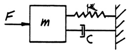 (Figure 1)
 (Figure 2)
 (Figure 3)
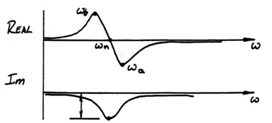 (Figure 4)
 (Figure 5)
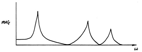 (Figure 6)
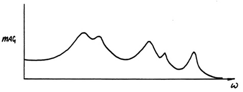 (Figure 7)
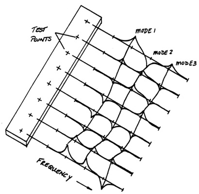 (Figure 8)
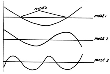 (Figure 9)
 for n = 1, ... ¥